# Control
# Overview
### General structure
The general structure of how the control system is made, tested, and deployed works like this:
The control system is made using Simulink, using mostly the base functionality to calculate the needed values for different parts of control. Once the general control system is implemented, it is either tested directly in Simulink, mostly using different parts from the Simscape suite to simulate the hardware, or it can be tested by generating the code, and using that code in a separate, more high level simulation program like Gazebo or Webots.
The deployment is mostly managed by the embedded team, as once the code is generated, it can be used in whatever is necessary for the embedded team.
### Required software
MATLAB Simulink with the following add-ons:
- Embedded Coder
- Simulink Coder
- Simulink Compiler
- MATLAB Coder
- MATLAB Compiler
### Code generation
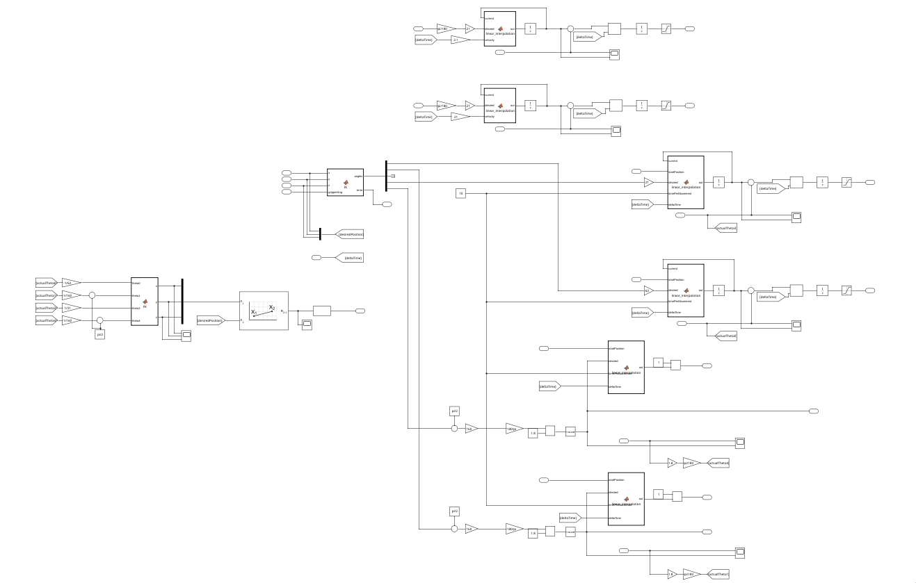
In general the code is generated from Simulink blocks, where all the control has to do is done inside this one block:
[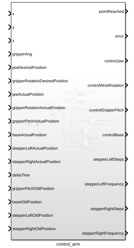](https://bookstack.roboteamtwente.nl/uploads/images/gallery/2026-04/L7Aimage.png)
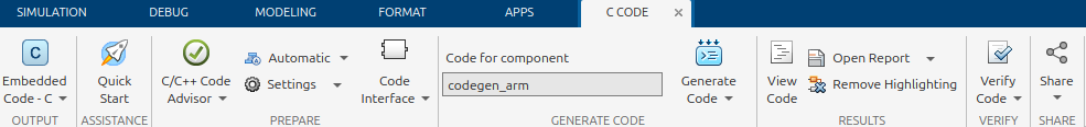
To be able to generate C code for the STM32's you will first need to activate the embedded C coder, which can be done by clicking on the apps tab in the top bar, and then searching for C embedded coder in the apps bar.
[](https://bookstack.roboteamtwente.nl/uploads/images/gallery/2026-04/WZEimage.png)
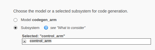
After the embedded C coder is active, a new tab called C CODE appears, where you now have to press the quick start button to start the code generation process:
[](https://bookstack.roboteamtwente.nl/uploads/images/gallery/2026-04/k84image.png)
When in the quick start menu, the only critical options for this project are to set the system which gets generated to the main control block of this project, and to set the word size to be the same as the ones from the STM32.
[](https://bookstack.roboteamtwente.nl/uploads/images/gallery/2026-04/Cvnimage.png)
[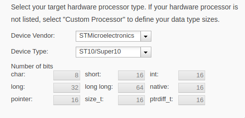](https://bookstack.roboteamtwente.nl/uploads/images/gallery/2026-04/isOimage.png)
The rest of the settings work best on the default option, but can be changed if deemed necessary.
# Automatic control
### Overview
In general, the job of the control system is to turn high level instructions from the software system, and turn them into instructions for the hardware. This is done by having a positions in 3d space (x, y z), a final gripper angle (respective to the ground), controls for the rotation, controls for opening and closing the gripper, and a deltaTime as an input, and turning those into control signals for the motors:
[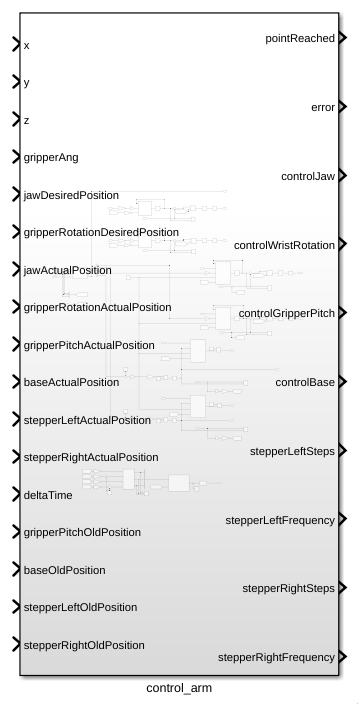](https://bookstack.roboteamtwente.nl/uploads/images/gallery/2026-04/UU3image.png)
The control system also has feedback from the motors with variables with a name ending with ActualPosition, and the old positions of the motors, representing the position of the motors before the movement starts.
[](https://bookstack.roboteamtwente.nl/uploads/images/gallery/2026-04/E9Pimage.png)
The movement starts whenever the input variables are changed, the old positions must come from an external source, and stay constant throughout the movement.
### Inverse kinematics
Starting of the process is the inverse kinematics, which is a matlab function block that calculates the necessary angles that the joints need to make given a final position.
[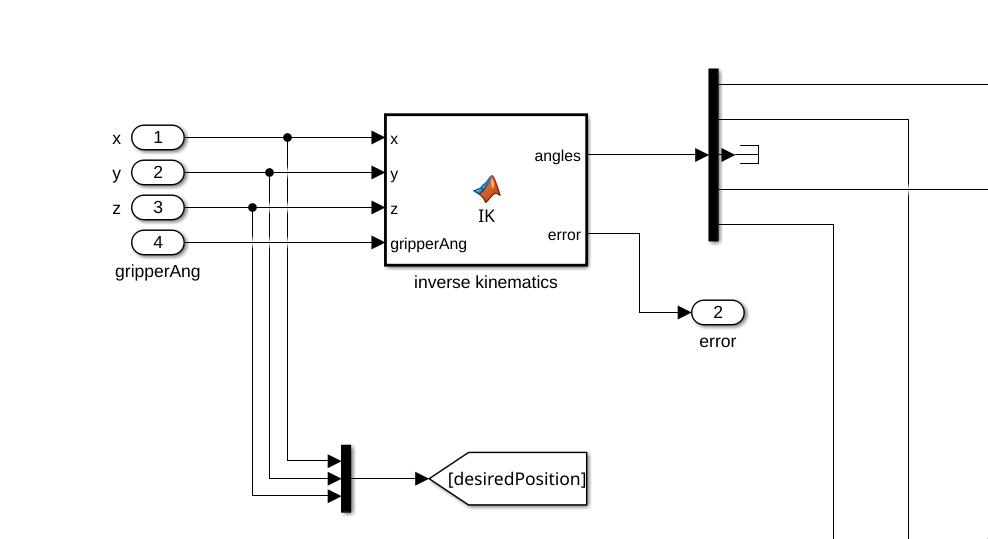](https://bookstack.roboteamtwente.nl/uploads/images/gallery/2026-04/a55image.png)
More information about how the inverse kinematics are done can be found in [Kinematics](https://bookstack.roboteamtwente.nl/books/robotic-arm/page/kinematics "Kinematics").
After that, angles will be sent to the different motor control systems, where they will be processes as a desired position.
[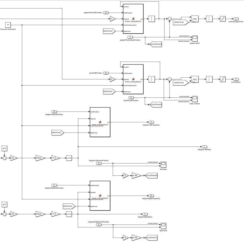](https://bookstack.roboteamtwente.nl/uploads/images/gallery/2026-04/h6cimage.png)
Here you will find a Time per movement constant, that will determine the speed at which a movement will be made. This is necessary to allow the motors to finish a movement at the same time, to minimize positioning issues.
#### Control signals
#### DC motors
The controllers used for DC motor control use a matlab function to linearly interpolate the movement, to allow for a smooth movement. It uses a start position, end position, and current position do determine how fast the motor should move.
[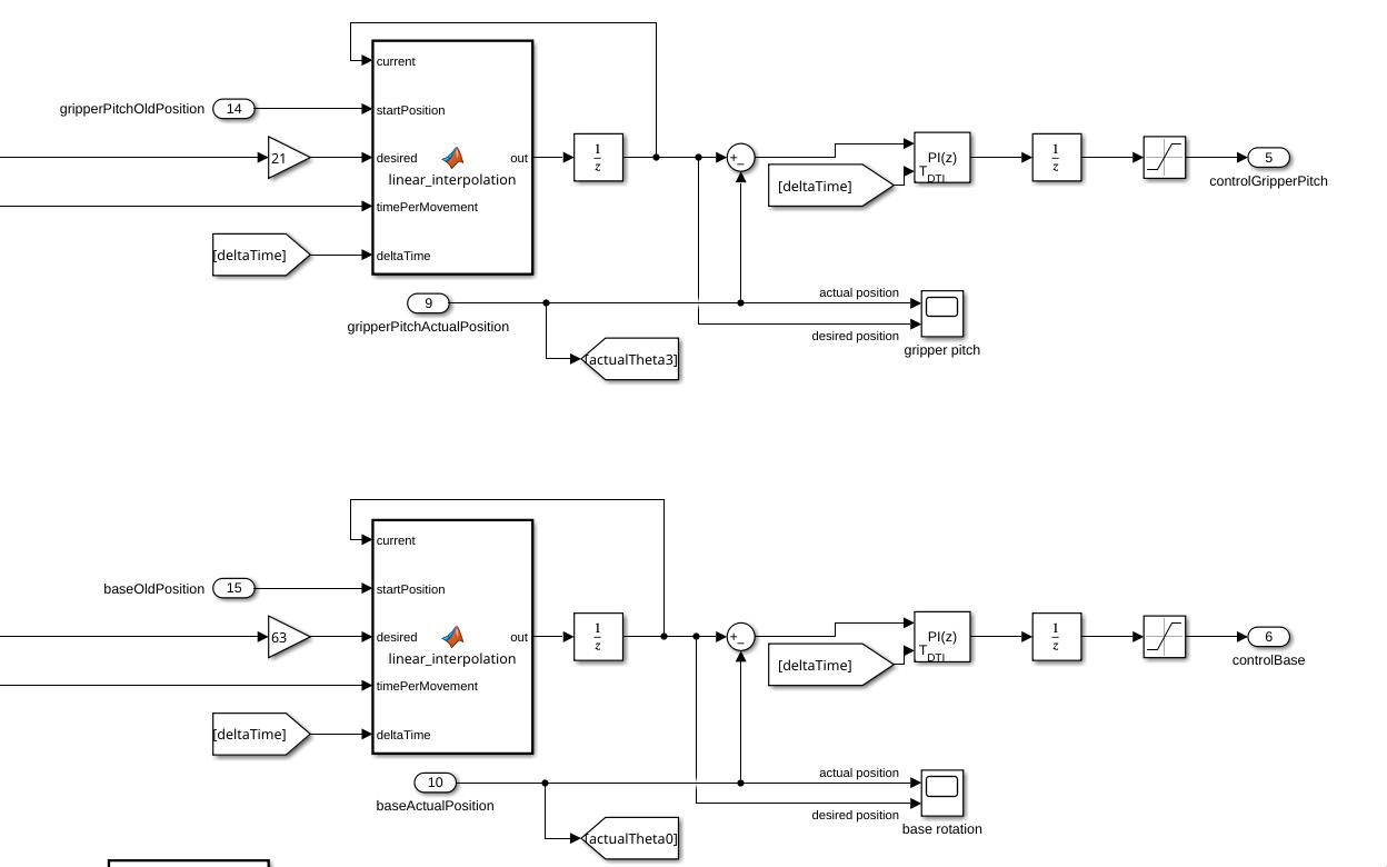](https://bookstack.roboteamtwente.nl/uploads/images/gallery/2026-04/WQximage.png)
The gain blocks going into the desired inputs are used to take into account the gearboxes attached to these motors (21:1 gear ratio means move 21 times further).
After the linear interpolation, the motor will be controlled using simple PI controllers, using the actual position from the encoders as control input. The actual positions will also be used for forward kinematics later, so they are sent to goto statements.
The linear interpolation works like this:
```matlab
function out = linear_interpolation(current, startPosition, desired, timePerMovement, deltaTime)
velocity = abs(desired - startPosition) / timePerMovement;
if current < desired
current = current + (velocity * deltaTime);
end
if current > desired
current = current - (velocity * deltaTime);
end
out = current;
```
The motors not used for positioning of the gripper (gripper rotation and jaw control) are also controlled using a linearly interpolated signal, but the velocity of these movements can be varied much more, because they are not dependent on the movement of the rest of the arm.
[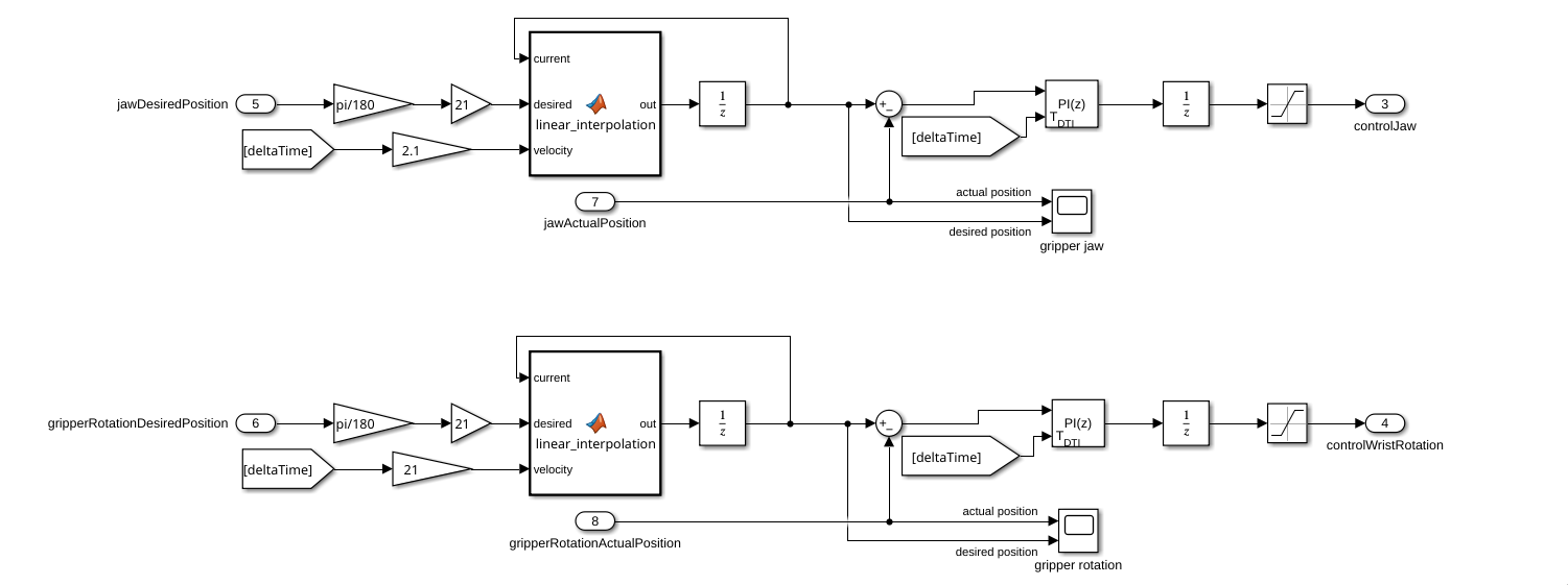](https://bookstack.roboteamtwente.nl/uploads/images/gallery/2026-04/v6Oimage.png)
After the linear interpolation, the motors are controlled with PI controllers.
The gain blocks in front of the desired position are scaled to account for an input of degrees, and to account for the gear ratios of the motors. The velocities were arbitrarily picked.
The linear interpolation block works like this:
```matlab
function out = linear_interpolation(current, desired, velocity)
if current < desired
current = current + velocity;
end
if current > desired
current = current - velocity;
end
out = current;
```
#### Stepper motors
The stepper motor control works fairly similar, but instead of sending control signals with a PI controller, it just sends the absolute position in terms of steps and the frequency at which the PWM signal should pulse.
[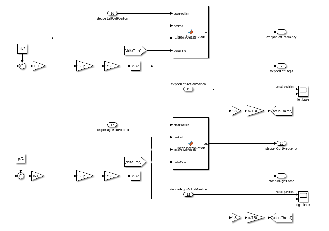](https://bookstack.roboteamtwente.nl/uploads/images/gallery/2026-04/beiimage.png)
Before getting the desired position though, three gain block are used beforehand, to convert the angle gotten from the inverse kinematics to the position the motor should go to. In this process a, pi/2 gets added to the angle because of how they are calculated.
The gain blocks are here for this reason: 160 is because of the gear ratio between the motor and the actual movement, 180/pi is to convert from radians to degrees, and 1/1.8 is to convert from degrees to steps (these could have been one gain block, but it is more clear why they are here like this).
The frequency calculating function block works like this:
```matlab
function out = linear_interpolation(startPosition, desired, timePerMovement, deltaTime)
velocity = abs(desired - startPosition) / timePerMovement;
out = velocity;
```
To confirm the robotic arm has reached the final position it has to, a forward kinematics function is used to get the projected position, which is then compared to the desired position.
[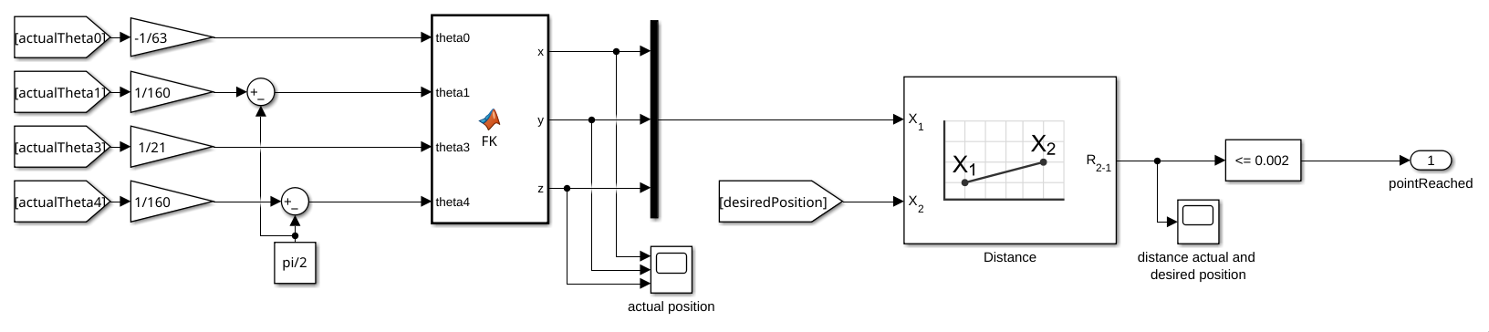](https://bookstack.roboteamtwente.nl/uploads/images/gallery/2026-04/9rVimage.png)
It does forward kinematics on the read values from the encoders, for that reason they have been scaled down to account for the gear ratios (pi/2 is subtracted from theta1 and theta4 because how the encoders are calibrated).
More on how the forward kinematics actually works in [Kinematics](https://bookstack.roboteamtwente.nl/books/robotic-arm/page/kinematics "Kinematics").
# Manual control
# Kinematics
### Defining terms
To do kinematics on the robotic arm, it first needs to be modelled in a way to do calculations on the different joint angles and positions. This is done by using [4x4 matrix notation](https://www.brainvoyager.com/bv/doc/UsersGuide/CoordsAndTransforms/SpatialTransformationMatrices.html) to represent the different joints.
The different points and angles are defined like this:
[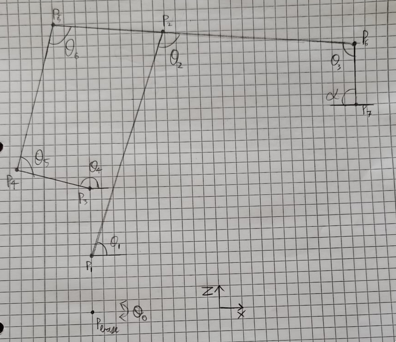](https://bookstack.roboteamtwente.nl/uploads/images/gallery/2026-04/Ojuimage.png)
In the all the following code blocks, there will be different types of variables used.
Variables that start with a P represent points,
variables that start with a T represent transform that can be performed on points,
and variables that start with an L are scalar length values.
Note: all angles are measured in radians, and all lengths are measured in meters.
### Forward kinematics
The input arguments of the function are the actuated angles of the arm, since these are the only ones measurable by the encoders.
The function returns the projected end position of the end effector.
```matlab
function [x, y, z] = forward_kinematics(theta0, theta1, theta3, theta4)
%defining dimentions
LbaseToP1 = 0.065;
LbaseToP3 = 0.149;
LP1toP2 = 0.350;
LP5toP6 = 0.620;
LP5toP2 = 0.120;
LP6toP7 = 0.300;
LP3toP4 = 0.120;
LP4toP5 = 0.280;
```
The first thing that happens in the forward kinematics is the definition of the dimensions of the different joints, these values are gotten from measuring the physical arm.
The point representing the base rotation (Pbase) is rotated theta0 radians.
```matlab
%rotation z
TP0toPbase = [cos(theta0) -sin(theta0) 0 0;
sin(theta0) cos(theta0) 0 0;
0 0 1 0;
0 0 0 1];
```
From there, all the known transforms to the different points are defined, the transforms are defined with the main idea being, rotation happens along the Z-axis, and translation happens along the X-axis. This is done by first translating shoulder actuated points (P1 and P3) and then rotating them along the x axis.
```matlab
%translation z then rotation x
TPbasetoP1 = [1 0 0 0;
0 0 -1 0;
0 1 0 LbaseToP1;
0 0 0 1];
%rotation z
TPbasetoP1 = TPbasetoP1 * [cos(theta1) -sin(theta1) 0 0;
sin(theta1) cos(theta1) 0 0;
0 0 1 0;
0 0 0 1];
```
```matlab
%translation z then rotation x
TPbasetoP3 = [1 0 0 0;
0 0 -1 0;
0 1 0 LbaseToP3;
0 0 0 1];
%rotation z
TPbasetoP3 = TPbasetoP3 * [cos(theta4) -sin(theta4) 0 0;
sin(theta4) cos(theta4) 0 0;
0 0 1 0;
0 0 0 1];
```
The reason that they are rotated twice is because it is easier to keep track of the relative positions and angles involved.
After that, the other currently inferrable transforms are defined.
```matlab
%translation x
TP1toP2 = [1 0 0 LP1toP2;
0 1 0 0;
0 0 1 0;
0 0 0 1];
%translation x then rotation z
TP5toP6 = [cos(theta3) -sin(theta3) 0 LP5toP6;
sin(theta3) cos(theta3) 0 0;
0 0 1 0;
0 0 0 1];
%translation x
TP6toP7 = [1 0 0 LP6toP7;
0 1 0 0;
0 0 1 0;
0 0 0 1];
%translation x
TP3toP4 = [1 0 0 LP3toP4;
0 1 0 0;
0 0 1 0;
0 0 0 1];
```
Some of these transforms don't have rotations, this is because we either don't know the angle rotation yet, or it is an end point, that does not have to be moved and by extension rotated further.
Due to the construction of the arm, some calculations have to be done to find the rest of the unknown angles.
This is done by first defining an initial position, and then some theoretical "planar" positions of the points P2 and P4.
```matlab
%initial position
P0 = [1 0 0 0;
0 1 0 0;
0 0 1 0;
0 0 0 1];
%getting position for paralellagram angles
P2planar = P0 * TPbasetoP1 * TP1toP2;
P4planar = P0 * TPbasetoP3 * TP3toP4;
```
The reason they are planar is because they were produces without any base rotation, so they all lay on the y=0 plane.
After that, a small inverse kinematics equation is performed to find the angles theta5 and theta6, which is done using a standard formula.
```matlab
L_1 = LP4toP5; L_2 = LP5toP2;
XE = P4planar(1, 4) - P2planar(1, 4);
YE = P4planar(3, 4) - P2planar(3, 4);
theta5 = 2*atan((2*L_1*YE + sqrt(- L_1^4 + 2*L_1^2*L_2^2 + 2*L_1^2*XE^2 + 2*L_1^2*YE^2 - L_2^4 + 2*L_2^2*XE^2 + 2*L_2^2*YE^2 - XE^4 - 2*XE^2*YE^2 - YE^4))/(L_1^2 + 2*L_1*XE - L_2^2 + XE^2 + YE^2));
theta6 = -2*atan(sqrt((- L_1^2 + 2*L_1*L_2 - L_2^2 + XE^2 + YE^2)*(L_1^2 + 2*L_1*L_2 + L_2^2 - XE^2 - YE^2))/(- L_1^2 + 2*L_1*L_2 - L_2^2 + XE^2 + YE^2));
%adding pi-theta4 to make the actual rotation angle
theta5 = theta5+(pi-theta4);
```
Now that we know all the angles, the rest of the transforms can be defined.
```matlab
%translation x then rotation z
TP3toP4 = [cos(theta5) -sin(theta5) 0 LP3toP4;
sin(theta5) cos(theta5) 0 0;
0 0 1 0;
0 0 0 1];
%translation x then rotation z
TP4toP5 = [cos(theta6) -sin(theta6) 0 LP4toP5;
sin(theta6) cos(theta6) 0 0;
0 0 1 0;
0 0 0 1];
```
And now we have all the transforms, we can calculate all the points.
```matlab
%calculating all needed points
Pbase = TP0toPbase;
P3 = Pbase * TPbasetoP3;
P4 = P3 * TP3toP4;
P5 = P4 * TP4toP5;
P6 = P5 * TP5toP6;
P7 = P6 * TP6toP7;
```
Finally, the final position of the end effector can be read from the final point.
```matlab
%extracting position
x = P7(1,4);
y = P7(2,4);
z = P7(3,4);
end
```
### Inverse kinematics
The inverse kinematics uses the same representation of points and angles to represent the linkages of the arm.
[](https://bookstack.roboteamtwente.nl/uploads/images/gallery/2026-04/6H1image.png)
The inputs for this function are the position of the end effector (x, y, z) and a final gripper angle alpha, which is in reference to the ground.
The outputs are the angles of the actuated points as shown above.
The first thing the function does checking a simple error case, as this will not be caught anywhere else otherwise.
```matlab
function [theta0, theta1, theta3, theta4, error] = inverse_kinematics(x, y, z, alpha)
defaultAngles = [0; pi/2; 0; -pi/2; pi];
error = 0;
if x == 0 && y == 0
theta0 = defaultAngles(1);
theta1 = defaultAngles(2);
%theta2 = defaultAngles(3);
theta3 = defaultAngles(4);
theta4 = defaultAngles(5);
error = 1;
return;
end
```
After that the same dimensions as the forward kinematics are defined.
```matlab
%all the lengths are in meters
LbaseToP1 = 0.065;
LbaseToP3 = 0.149;
LP1toP2 = 0.350;
LP2toP6 = 0.500;
%LP5toP6 = 0.620;
LP5toP2 = 0.120;
LP6toP7 = 0.300;
LP3toP4 = 0.120;
LP4toP5 = 0.280;
```
Since the arm is planar by nature, the angle of the base rotation (theta0) can easily be calculated. A variable called angToBase is also defined, it represents the angle of the end effector to the base of the arm.
```matlab
if x < 0
theta0 = atan(y/x) + pi;
else
theta0 = atan(y/x);
end
angToBase = theta0 - pi;
```
After that, P7 and P6 are defined using the input arguments. The rotation x on P7 is to align rotations with the z-axis and translations with the x-axis. (The i at the end is for inverse.)
```matlab
%setting end position, rotated towards the base
P7i = [cos(angToBase) -sin(angToBase) 0 x;
sin(angToBase) cos(angToBase) 0 y;
0 0 1 z;
0 0 0 1];
%rotation x
P7i = P7i * [1 0 0 0;
0 0 -1 0;
0 1 0 0;
0 0 0 1];
%rotation z
TP7toP6i = [cos(alpha) -sin(alpha) 0 0;
sin(alpha) cos(alpha) 0 0;
0 0 1 0;
0 0 0 1];
%translation x
TP7toP6i = TP7toP6i * [1 0 0 LP6toP7;
0 1 0 0;
0 0 1 0;
0 0 0 1];
P6i = P7i * TP7toP6i;
```
P1 is also defined.
```matlab
%translation z
P1i = [1 0 0 0;
0 1 0 0;
0 0 1 LbaseToP1;
0 0 0 1];
```
Now that P1, P6, and P7 are defined, they will be used to calculate theta1, theta2, and theta3.
This is done by first checking if this movement would be possible kinematically, and then actually calculating the angles. This is done with the same standard formula shown in the forward kinematics.
```matlab
%calculating theta1, theta2 and theta3
L_1i = LP1toP2; L_2i = LP2toP6;
dx = P6i(1,4) - P1i(1,4);
dy = P6i(2,4) - P1i(2,4);
XEi = sqrt(dx*dx + dy*dy);
YEi = P6i(3,4) - P1i(3,4);
if (- L_1i^4 + 2*L_1i^2*L_2i^2 + 2*L_1i^2*XEi^2 + 2*L_1i^2*YEi^2 - L_2i^4 + 2*L_2i^2*XEi^2 + 2*L_2i^2*YEi^2 - XEi^4 - 2*XEi^2*YEi^2 - YEi^4) < 0
error = 1;
theta0 = defaultAngles(1);
theta1 = defaultAngles(2);
%theta2 = defaultAngles(3);
theta3 = defaultAngles(4);
theta4 = defaultAngles(5);
return;
end
theta1 = 2*atan((2*L_1i*YEi + sqrt(- L_1i^4 + 2*L_1i^2*L_2i^2 + 2*L_1i^2*XEi^2 + 2*L_1i^2*YEi^2 - L_2i^4 + 2*L_2i^2*XEi^2 + 2*L_2i^2*YEi^2 - XEi^4 - 2*XEi^2*YEi^2 - YEi^4))/(L_1i^2 + 2*L_1i*XEi - L_2i^2 + XEi^2 + YEi^2));
theta2 = -2*atan(sqrt((- L_1i^2 + 2*L_1i*L_2i - L_2i^2 + XEi^2 + YEi^2)*(L_1i^2 + 2*L_1i*L_2i + L_2i^2 - XEi^2 - YEi^2))/(- L_1i^2 + 2*L_1i*L_2i - L_2i^2 + XEi^2 + YEi^2));
theta3 = 2*pi - alpha -theta1 -theta2;
```
These angles are then used to define transforms to other necessary points. An initial point is also defined.
```matlab
%translation z then rotation x
TPbasetoP1 = [1 0 0 0;
0 0 -1 0;
0 1 0 LbaseToP1;
0 0 0 1];
%rotation z
TPbasetoP1 = TPbasetoP1 * [cos(theta1) -sin(theta1) 0 0;
sin(theta1) cos(theta1) 0 0;
0 0 1 0;
0 0 0 1];
%translation x then rotation z
TP1toP2 = [cos(theta2) -sin(theta2) 0 LP1toP2;
sin(theta2) cos(theta2) 0 0;
0 0 1 0;
0 0 0 1];
%translation z then rotation x
TPbasetoP3 = [1 0 0 0;
0 0 -1 0;
0 1 0 LbaseToP3;
0 0 0 1];
%translation x
TP2toP5 = [1 0 0 -LP5toP2;
0 1 0 0;
0 0 1 0;
0 0 0 1];
%initial position
P0 = [1 0 0 0;
0 1 0 0;
0 0 1 0;
0 0 0 1];
```
These new transforms are now used to interpolate planar versions of P3 and P5.
```matlab
%getting position for paralellagram angles
P3planar = P0 * TPbasetoP3;
P5planar = P0 * TPbasetoP1 * TP1toP2 * TP2toP5;
```
These points are used to calculate the final needed angles, using the same formula as before.
```matlab
%getting parallelageram angles
L_1 = LP3toP4; L_2 = LP4toP5;
XE = P5planar(1, 4) - P3planar(1, 4);
YE = P5planar(3, 4) - P3planar(3, 4);
if (- L_1^4 + 2*L_1^2*L_2^2 + 2*L_1^2*XE^2 + 2*L_1^2*YE^2 - L_2^4 + 2*L_2^2*XE^2 + 2*L_2^2*YE^2 - XE^4 - 2*XE^2*YE^2 - YE^4) < 0
error = 1;
theta0 = defaultAngles(1);
theta1 = defaultAngles(2);
%theta2 = defaultAngles(3);
theta3 = defaultAngles(4);
theta4 = defaultAngles(5);
return;
end
theta4 = 2*atan((2*L_1*YE + sqrt(- L_1^4 + 2*L_1^2*L_2^2 + 2*L_1^2*XE^2 + 2*L_1^2*YE^2 - L_2^4 + 2*L_2^2*XE^2 + 2*L_2^2*YE^2 - XE^4 - 2*XE^2*YE^2 - YE^4))/(L_1^2 + 2*L_1*XE - L_2^2 + XE^2 + YE^2));
```
Note: the angles resulting from the function are equal to the angles defined on the diagram above, which are not equal to the positions the motors have to move to.
# Simulation
### Simulink
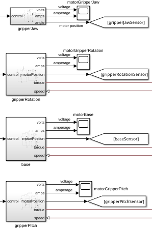
#### Overview
The main simulation used for testing the control system of the robotic arm is made with Simulink, using the different parts of the Simscape suite to simulate the robotic arm.
[](https://bookstack.roboteamtwente.nl/uploads/images/gallery/2026-04/BiWimage.png)
The simulation works by using a main control block that sends instructions to different simulated motors, which are then connected to a 3d model of the robotic arm.
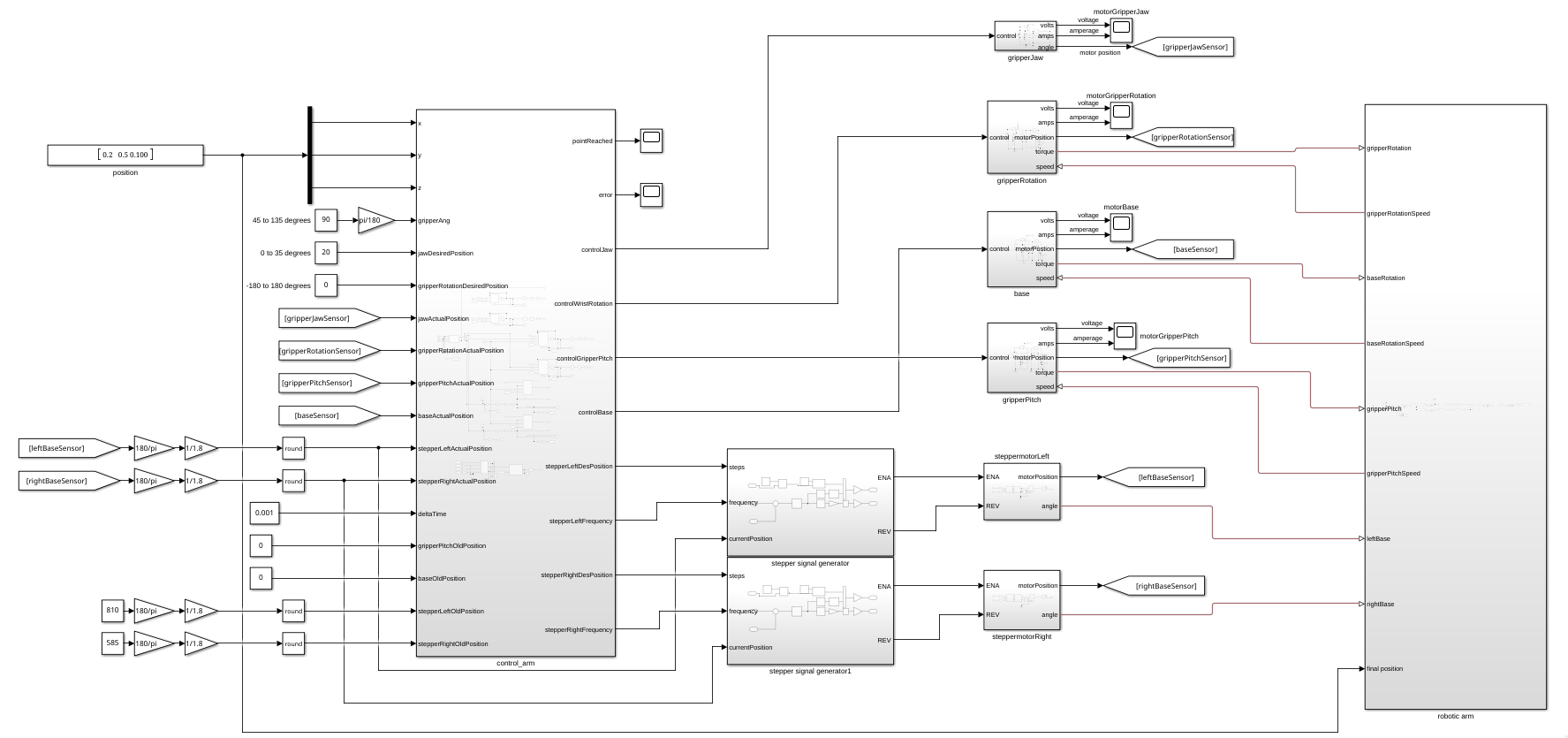
#### Motors
There are two main types of motors used for simulation, DC motors and stepper motors. All of these parts are simulated using the Simscape suite.
##### DC motors
The parts controlled by DC motors are the base rotation, gripper pitch, gripper rotation, and gripper jaw (opening and closing).
[](https://bookstack.roboteamtwente.nl/uploads/images/gallery/2026-04/xdcimage.png)
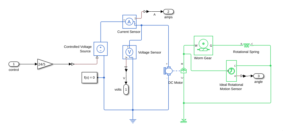
The DC motors are controlled with a control signal that ranges from 0V-5V, which is then converted to a 0V-24V signal that the motor can use. The voltage and amperage going to the motor are measured and sent to outputs to get estimations of how much power the motors will use.
[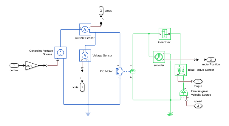](https://bookstack.roboteamtwente.nl/uploads/images/gallery/2026-04/qHVimage.png)
The resulting rotational force is then sent to a gearbox, after which the torque sensor and angular velocity source are used to connect the motor to the model of the arm. The toque sensor is connected to the torque inputs of the joints, and the velocity source is connected to the speed output of the joints.
[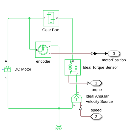](https://bookstack.roboteamtwente.nl/uploads/images/gallery/2026-04/Vhjimage.png)
The position of the motor is measured before the gearbox, as this is where the encoder would be on the actual motors.
Since the jaw motors is not currently simulated to move the model of the arm, it has its own simple implementation that takes into account the resistance of the springs that are on the jaws of the gripper.
[](https://bookstack.roboteamtwente.nl/uploads/images/gallery/2026-04/M5bimage.png)
It uses a worm gear and a spring to simulate how the jaws would move without anything in them.
##### Stepper motors
The two motors in the shoulder joint, actuating the parallelogram construction are stepper motors. These are controlled in two stages, first determining the desired position in terms of steps and the frequency at which the steps should happen, and then generating the steps to make the stepper motors move.
[](https://bookstack.roboteamtwente.nl/uploads/images/gallery/2026-04/i2Pimage.png)
The role of the stepper signal generators is to generate a PWM signal as the STM32's would do given the absolute position and frequency of the steps.
[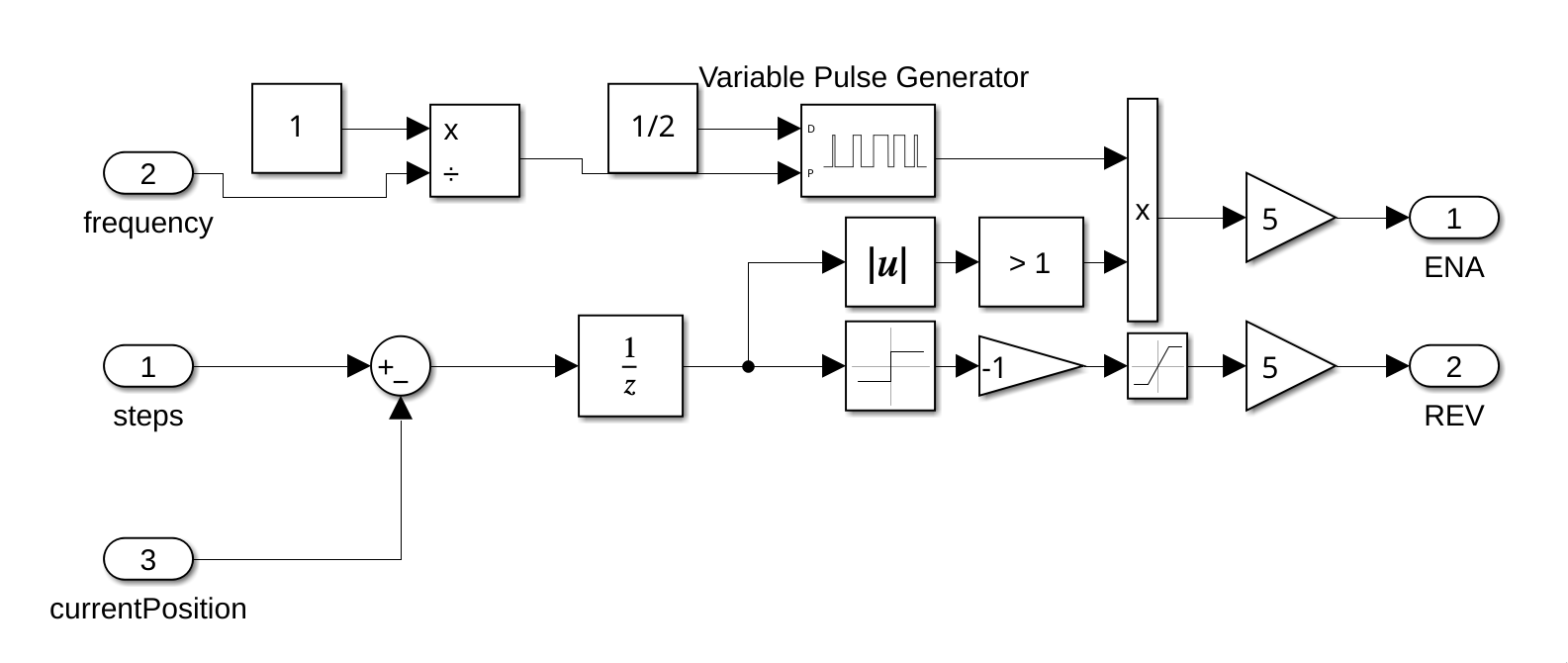](https://bookstack.roboteamtwente.nl/uploads/images/gallery/2026-04/S99image.png)
Simply what it does is send pulses at the specified frequency whenever the error between the desired step position is different from the real one.
Note: this way of generating pulses is only for this specific simulation, and would be a bad implementation for anything else.
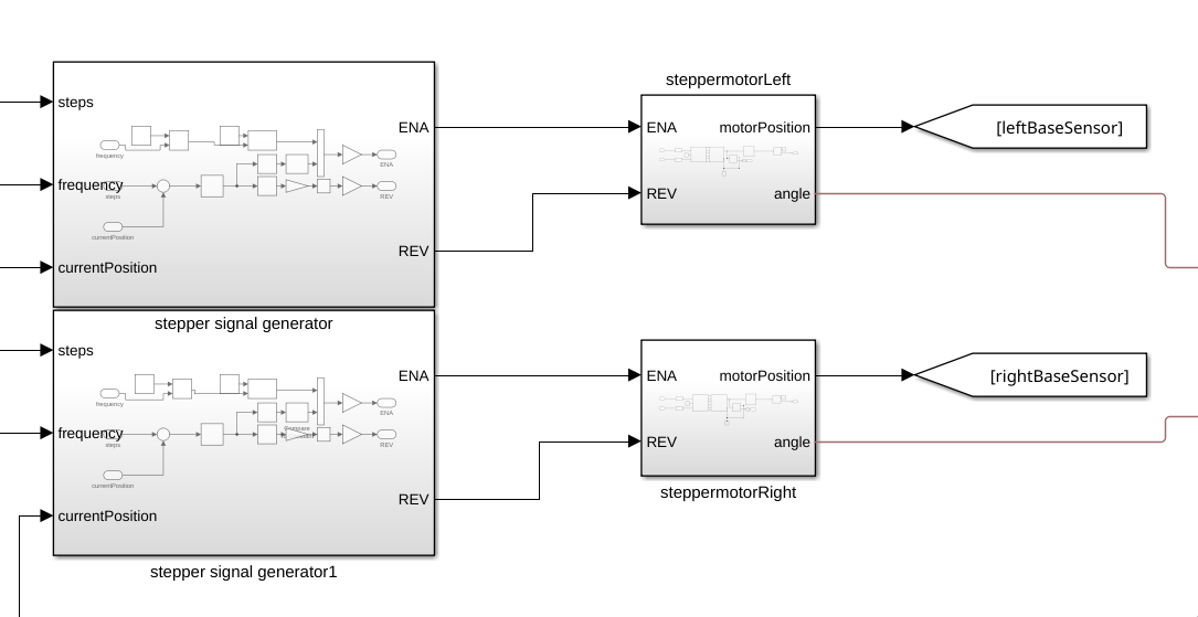
The stepper motors work by connecting the ENA and REV connections from the previous block to the ENA and REV from a stepper motor driver, which makes the stepper motor move.
[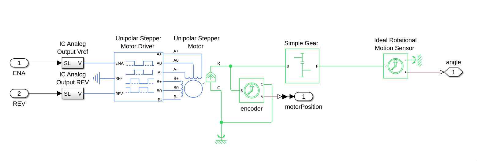](https://bookstack.roboteamtwente.nl/uploads/images/gallery/2026-04/E1Zimage.png)
The rotational movement from the stepper motor is read both before and after the gearbox, before to get the encoder values from the motor, and after to use as output to the robotic arm model.
#### 3d model
To show a 3d simulation of the robotic arm, a simplified version of the arm is used. Most of the part models are ported from SolidWorks, using STEP files to render the models. Apart from the gripper, which uses an altered version of the gripper model, and uses two obj files, one for the base and one for the claw, to allow for rotation of the gripper in the simulation.
[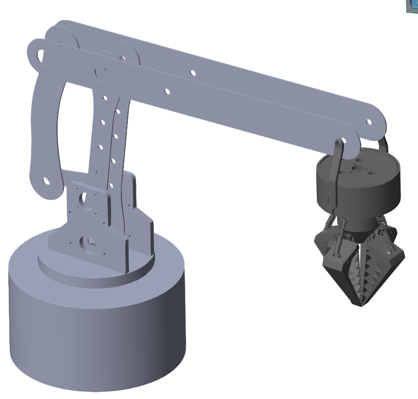](https://bookstack.roboteamtwente.nl/uploads/images/gallery/2026-04/I2qimage.png)This model is connected to the simulated motors by connecting the physical torque signals the motors produce, and connecting the output speed from the joints back to the motors. This allows the control system to send instructions to the motors, and let the motors then manipulate the arm.
In Simulink, the simulation of the robotic arm by connecting different Simscape parts together with different types of joints.
[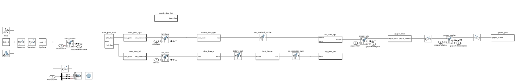](https://bookstack.roboteamtwente.nl/uploads/images/gallery/2026-04/CM0image.png)
Each of the white blocks are parts, and the joints, due to the nature of the arm, are all revolute joints.
[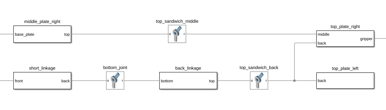](https://bookstack.roboteamtwente.nl/uploads/images/gallery/2026-04/stTimage.png)
The different parts work by having a rigid transform from one attachment point to the other, as well as a reference point and a model file, to show how the arm would actually look like.
[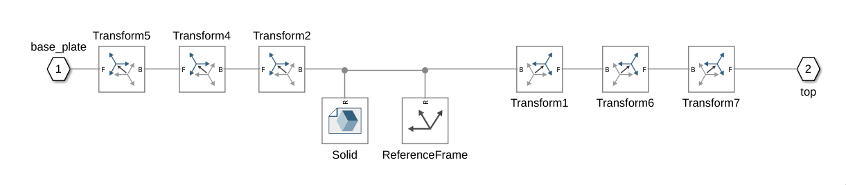](https://bookstack.roboteamtwente.nl/uploads/images/gallery/2026-04/i6timage.png)
The actuated joints are connected to connection points that connect to the motors from outside of the model block.
[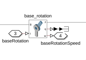](https://bookstack.roboteamtwente.nl/uploads/images/gallery/2026-04/xiqimage.png)
The model also includes a red ball that is moved to the desired position of the end effector, which in this case is the tip of the gripper.
[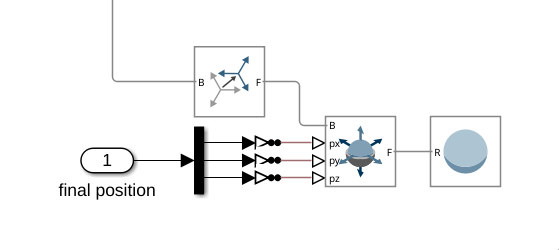](https://bookstack.roboteamtwente.nl/uploads/images/gallery/2026-04/HHOimage.png)
### Webots